Two years ago, I gave an LLM access to a simple Python API for programmatically generating vector images. Given the outlandish amount of progress in LLM coding capabilities, I wanted to figure out if a small model like Qwen3.5-4B with a simple coding harness could do the same.
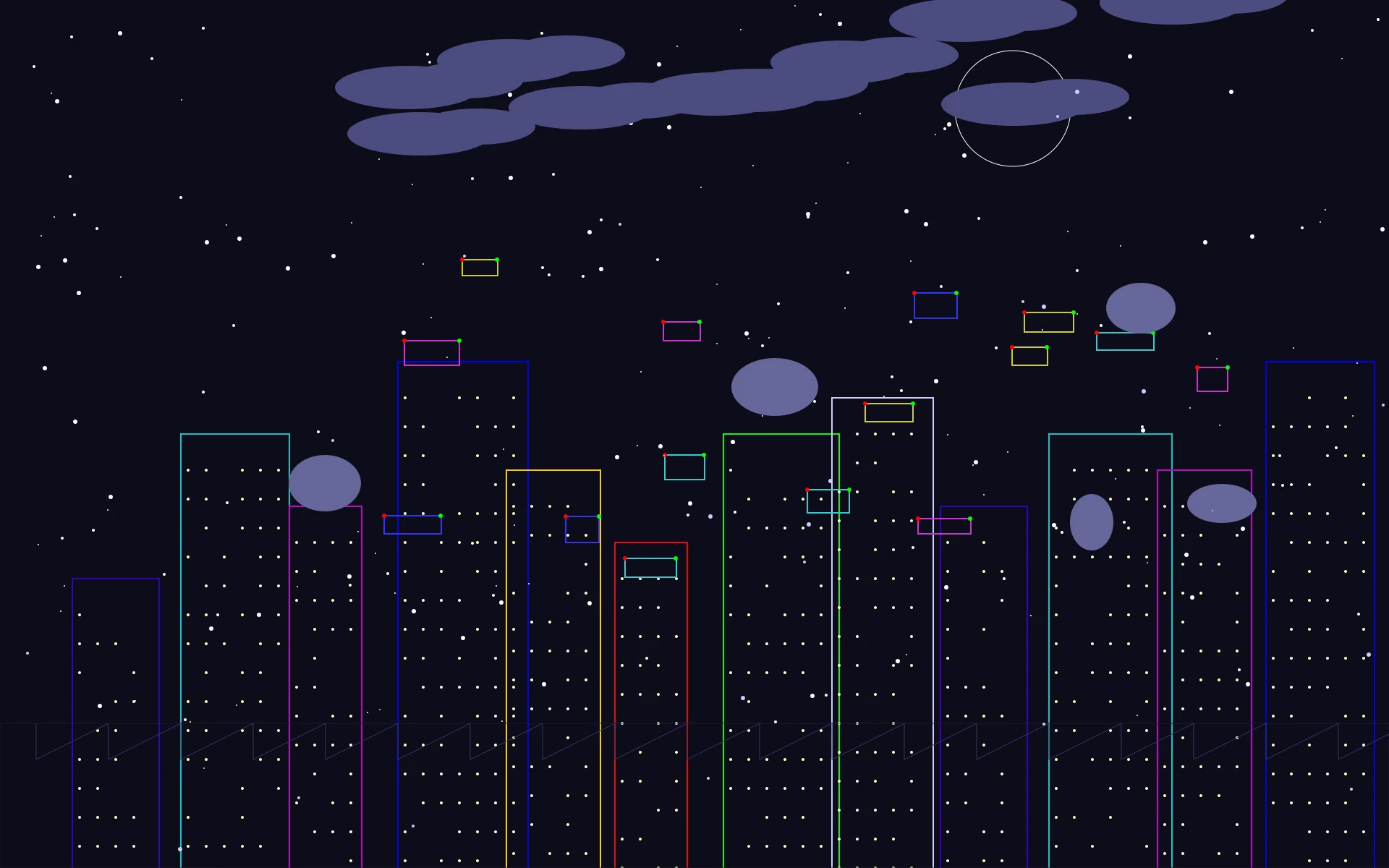
This was something, but I realised I could make it even better by fine-tuning the model. After many iterations and experiments, which I describe in the technical appendix, I came up with this training setup and the results below
- Base modelQwen3.5-4B
- Supervised fine-tuningLearn from a teacher model’s drawing traces
- Execution rewards (RLVR)Reward valid renders
- Preference training (RLHF)Score images with a preference model
Evaluation results
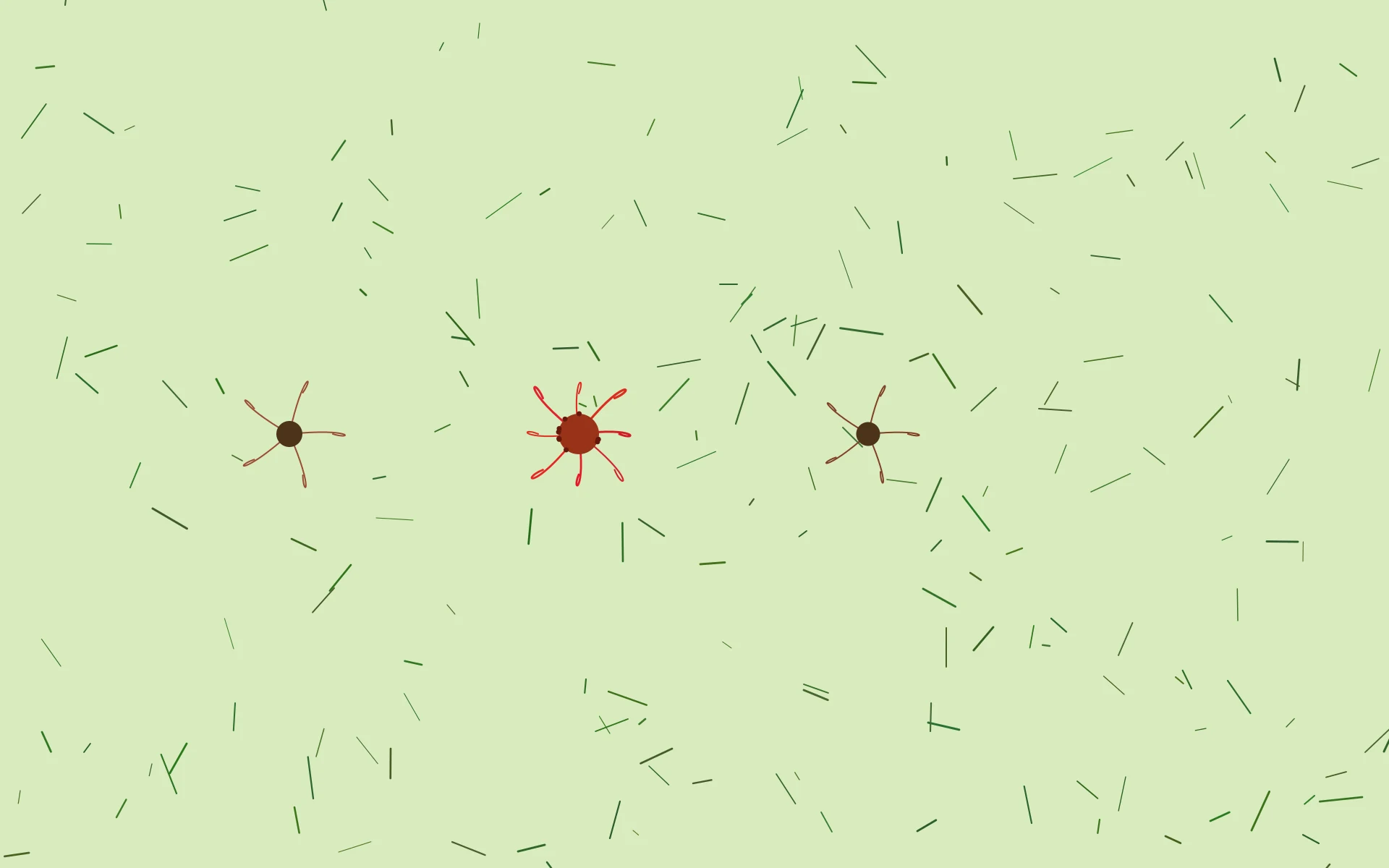
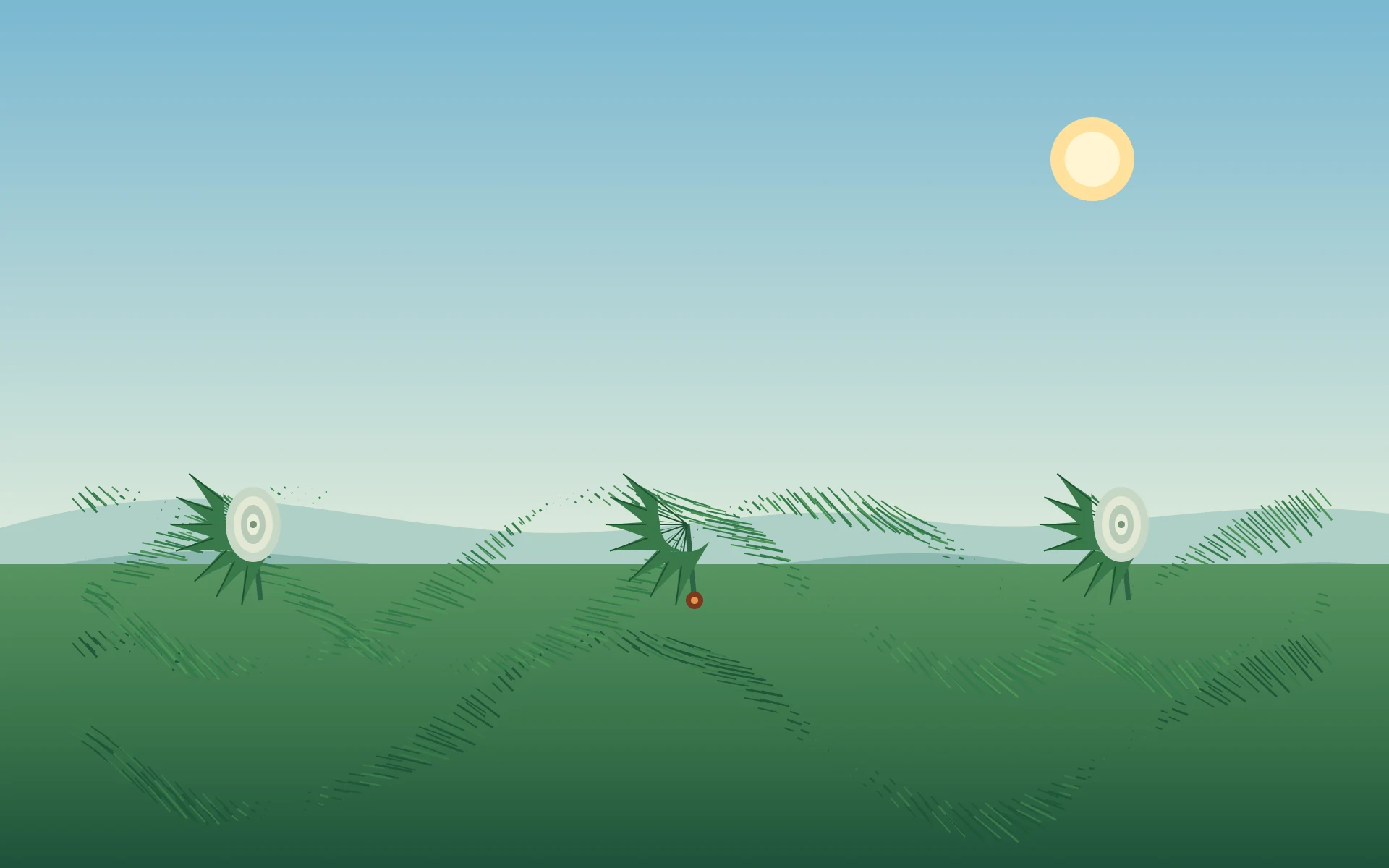


Try Artsy
I put the final model in this demo website.Try it out yourself!
Appendix
Harness and workflow
The original harness gave the model five custom drawing tools. In Experiment 5 I switched to mini-SWE-agent 2.2.3, with 2 additional custom tools. The model could make one call per turn. Each call started a new shell in the same Docker workspace. Files persisted across turns, while working-directory changes and environment exports lasted only for the current command.
| Action | Original | mini-SWE |
|---|---|---|
| Write and revise | update_drawing(source) replaced the entire Python program on each edit. | bash(command) could create files, run Python, or apply a focused edit with sed or patch. Files persisted across turns. |
| Inspect | read_drawing() returned the current Python source. | Shell utilities let the model read individual files, search with ripgrep, and compare versions with diff. |
| Preview | preview_drawing() ran the current source and returned execution feedback and, on success, the PNG. | artsy-preview accepted a PNG to display or a Python entrypoint to render. The model could see the image on its next turn. |
| Submit | submit_drawing() ended the episode and sent the current source for a fresh render. | artsy-submit ENTRYPOINT captured the entrypoint and its Python modules. The final renderer ran that code in a clean directory. |
| Decline | refuse_drawing(reason) ended the episode and recorded the reason. | I removed the refusal tool when I switched to drawing-only prompts. |
Recommended Workflow
- Write and run
rm -f output.png && python ENTRYPOINTUse the ArtCanvas reference in the prompt. Seed any randomness so both renders agree. - Inspect
artsy-preview output.pngView the existing PNG. Pass the Python entrypoint to rerun the code instead.Changes needed? Edit the code, then return to Write and run. - Preview looks rightSubmit
artsy-submit ENTRYPOINTBundle the entrypoint and local Python modules, up to 64 KiB, and end the episode. A preview on the last turn leaves no submission to score. - ScoreRerun the bundle in a fresh directory within 60 seconds. Count a delivery if the program exits successfully and writes a decodable 1920 × 1200
output.pngup to 8 MiB.
Original tool definitions · mini-SWE drawing instructions · Preview and submit commands · Final render implementation
ArtCanvas API reference
ArtCanvas is a simple drawing API the coding agent is given access to. It wraps Pycairo with a white canvas and a one-pixel black brush by default. The v2.1 signatures below come from the current runtime. Version 2.1 adds ellipses, clipping, patterns, reusable paths, and layers to the core v2 API. Coordinates and lengths are in pixels, and color channels and opacity are in the range 0–1. The constructor accepts integer dimensions from 1 to 4096. The drawing evaluator requires a 1920 × 1200 PNG.
from artcanvas import ArtCanvas

ArtCanvas(width=1920, height=1200, filename="output.png")

# Shapes, brush, and output
move_brush_to(x, y)
draw_line_to(x, y)
draw_arc(xc, yc, radius, start_angle, end_angle)
draw_rectangle(x, y, width, height, fill=False)
draw_rounded_rectangle(x, y, width, height, radius, fill=False)
draw_circle(x, y, radius, fill=False)
draw_ellipse(x, y, radius_x, radius_y, fill=False)
draw_polygon(points, fill=False)
draw_bezier_curve(x1, y1, cx1, cy1, cx2, cy2, x2, y2)
draw_text(x, y, text, font_size=16, font_family="Sans")
set_color(r, g, b, a=1.0)
set_line_width(width)
set_line_cap(cap)
set_line_join(join)
set_dash_pattern(dashes, offset=0)
fill_background(r, g, b)
save()

# Gradients and textures
set_gradient(x1, y1, x2, y2, stops)
set_radial_gradient(cx1, cy1, radius1, cx2, cy2, radius2, stops)
set_pattern(kind, spacing=8, angle=0, line_width=1,
            opacity=1, color=None, seed=0)
fill_pattern(kind, spacing=8, angle=0, line_width=1,
             opacity=1, color=None, seed=0)

# Paths and clipping
new_path()
move_to(x, y)
line_to(x, y)
curve_to(cx1, cy1, cx2, cy2, x, y)
ellipse_path(x, y, radius_x, radius_y)
close_path()
stroke()
fill()
stroke_preserve()
fill_preserve()
clip()
reset_clip()
create_path()
append_path(path)
draw_path(path, fill=False, stroke=False)

# Transforms and compositing
save_state()
restore_state()
translate(x, y)
rotate(radians)
scale(x, y)
begin_layer(opacity=1, blend_mode="over")
end_layer(blur_radius=0)
layer(opacity=1, blend_mode="over", blur_radius=0)- Brush and output. Gradient stops are
(offset, r, g, b, a)tuples. A polygon needs at least three(x, y)points. Line caps arebutt,round, orsquare. Line joins aremiter,round, orbevel.fill_background()resets the brush to black.save()writes the PNG and finishes the surface. The context manager calls it on successful exit. - Paths and clipping. Path commands build geometry for a later fill or stroke. The preserve variants keep the current path available.
clip()intersects the clip with the path and consumes it.create_path()copies the current geometry, anddraw_path(path)strokes it by default.save_state()andrestore_state()scope brush settings, transforms, and clipping. - Patterns. Choose
hatching,crosshatch,dots,stipple, ornoise. Pattern angles are in degrees. Arcs and rotation use radians. Pass an RGB or RGBA tuple to override the current solid brush color. Gradients fall back to black. Spacing ranges from 1 to 512 pixels, and the seed controls randomized stipple and noise.set_pattern()changes the brush source.fill_pattern()paints the current clip and restores the previous source. - Layers. Layers can nest and are composited when they close. Blend modes are
over,multiply,screen,overlay,add,darken, andlighten. The optional Gaussian blur accepts a radius from 0 to 100 pixels.with canvas.layer(...)pairs the begin and end calls.
Drawing example
This program fills an ellipse with a gradient, adds hatching inside the same shape, and composites a blurred highlight. The outer context manager writes output.png.
from artcanvas import ArtCanvas

with ArtCanvas() as canvas:
    canvas.fill_background(0.96, 0.94, 0.87)
    canvas.save_state()
    canvas.ellipse_path(960, 600, 440, 240)
    canvas.clip()
    canvas.set_gradient(520, 360, 1400, 840, [
        (0, 0.13, 0.42, 0.48, 1),
        (1, 0.04, 0.14, 0.22, 1),
    ])
    canvas.draw_rectangle(520, 360, 880, 480, fill=True)
    canvas.fill_pattern("hatching", spacing=9, angle=30,
                        opacity=0.20, color=(1, 1, 1))
    with canvas.layer(opacity=0.65, blend_mode="screen", blur_radius=12):
        canvas.set_color(0.7, 0.9, 0.8)
        canvas.draw_ellipse(850, 510, 160, 32, fill=True)
    canvas.restore_state()
ArtCanvas API guide · Python implementation
Data Generation
The first rank study used 1,763 demonstrations generated wit GPT-6 Luna from 906 distinct Parti prompts. I trained each adapter for one epoch with seed 42, batches of 32 trajectories, and a cosine schedule starting at 0.0002. All three runs took 56 updates. I generated one drawing per evaluation prompt at temperature zero, with the same seed across models, up to 25 turns and up to 32,768 output tokens per response.
The 391-prompt evaluation combined the original 163 prompts with 228 extra ones. I checked IDs and normalized text against the training input. Once I collected demonstrations for those 228 prompts in Experiment 3, only the original 163 remained held out. Of the 327 Parti prompts set aside for reinforcement learning, 227 went into the verifier runs and 100 into preference training.
For GenAI-Bench I used the prompts and skill labels from a pinned snapshot of BaiqiL/GenAI-Bench-1600. The hard evaluation had 50 prompts about counting and binding, 50 about spatial composition, and 50 about comparison and logic. Each prompt had at least three skill tags, and advanced tags counted extra in the selection score. The screening script normalizes case and whitespace, then flags exact token-string matches, token-set Jaccard similarity of 0.80 or more, and character similarity of 0.90 or more when length and vocabulary overlap also pass their thresholds. A paraphrase could still pass that check. The skill tags were my proxy for difficulty. Prompt selection and screening code
- Animals219 (19.2%)
- Artifacts200 (17.5%)
- World Knowledge149 (13.0%)
- People124 (10.9%)
- Outdoor Scenes93 (8.1%)
- Other357 (31.3%)
- Basic190 (16.6%)
- Simple Detail161 (14.1%)
- Fine-grained Detail217 (19.0%)
- Complex80 (7.0%)
- Style & Format144 (12.6%)
- Other350 (30.6%)
- 1–3344 (75.8%)
- 4–6101 (22.2%)
- 7–99 (2.0%)
- Counting and binding114 (25.1%)
- Spatial composition114 (25.1%)
- Comparison and logic113 (24.9%)
- Scene attributes113 (24.9%)
I counted deliveries across every prompt. For paired image judgments, I kept only prompts where both models submitted a valid drawing.
Training
The three published adapters use LoRA rank 128 and the same pinned Qwen3.5-4B base revision. I trained them with Tinker using seed 42. For preference training, both branches start independently from expanded RLVR. Both keep the SFT sampler as their frozen KL reference.
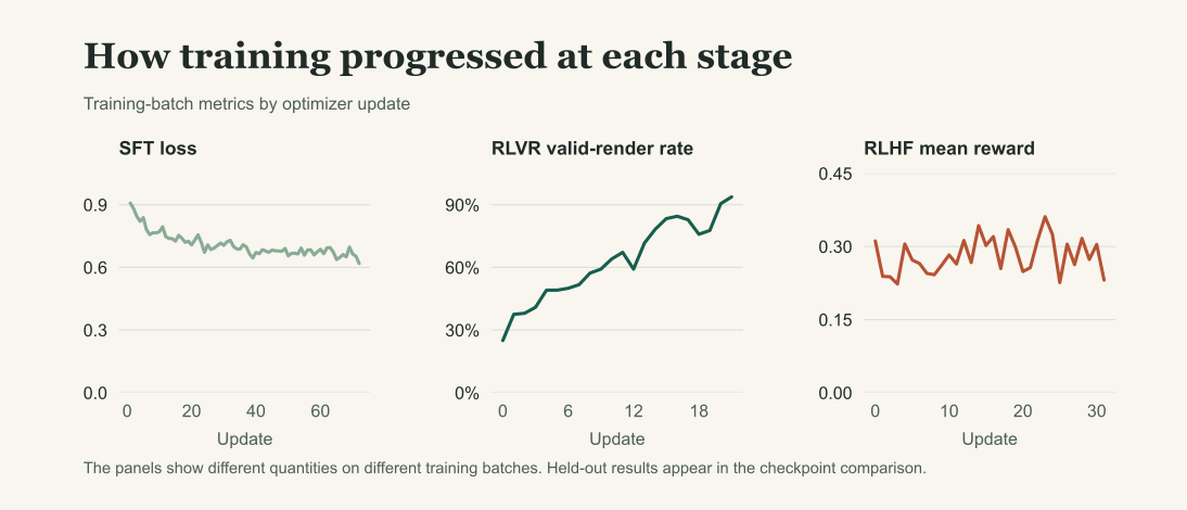
- SFT. I trained for one epoch on 2,282 Luna trajectories in batches of 32, with a cosine schedule starting at 0.0002. The mini-SWE export retains commands, text feedback, and preview pixels in conversation order. It applies loss to executed assistant actions across the cumulative edit sequence. The final manifest records 8,273 supervised actions over 72 updates. Trajectory conversion · SFT adapter card
- Expanded RLVR. I initialized from SFT update 72 and trained for one epoch on 681 prompts, with 32 prompt groups per full update and four rollouts per group. The verifier scores the final render, tool-call format, and shell execution. This produced the step-22 checkpoint used for both preference branches. Verifier code · RLVR adapter card
- Preference training. I used HPSv3 on the submitted render. The 300-prompt branch finished at update 10 and the 1,000-prompt branch finished at update 32. The final adapter is the 1,000-prompt branch. Final adapter card
Training plots
Supervised fine-tuning (SFT)
I used Luna’s tool-use traces as demonstrations for supervised fine-tuning. A trace shows how the teacher gets from a prompt to a finished drawing, including the code it writes and the previews it sees along the way.
Experiment 1. LoRA rank comparison
I trained rank-32, rank-64, and rank-128 adapters on the same 1,763 trajectories and tested them alongside the base model on 163 held-out PartiPrompts. I scored the submitted images with HPSv3, an image preference model. Each head-to-head comparison uses the prompts where both adapters delivered an image.
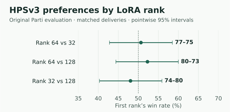



Research noteRank 128 had the highest mean HPSv3 reward across the 150 prompts all three adapters finished. The head-to-head comparisons were close, so the ranking was still open.
Experiment 2. Evaluation on 391 prompts
I added 228 prompts and kept the 25-turn limit. Rank 64 used about 1.61 fewer turns per prompt than rank 32. That difference held after correction for multiple comparisons. The adapters delivered similar numbers of images.
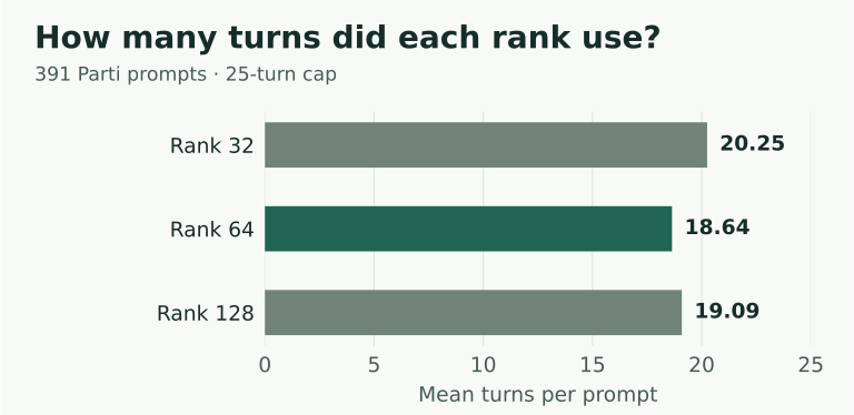
Research noteRank 64 was my provisional choice because it needed fewer turns than rank 32 in this evaluation. On the 205 new prompts all three adapters finished, Luna gave ranks 32 and 64 the same average visual-quality score. I still wanted to see what happened with more training examples.
Experiment 3. Fine-tuning with additional demonstrations
I moved those 228 additional prompts back into the SFT pool and collected 456 new Luna trajectories. I trained all three ranks again from the base model, this time on 2,219 trajectories, and evaluated on the original 163 held-out prompts. Ranks 32, 64, and 128 delivered 153, 156, and 153 images, respectively.
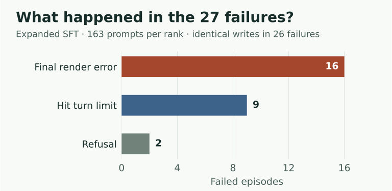
Research noteOn prompts both adapters finished, HPSv3 favored rank 128 over rank 64 by 81–65 and over rank 32 by 75–72. I ran one training seed per rank. The failed traces gave me something concrete to investigate. In 26 of 27 failures, the model wrote the same source code more than once. Each of the nine runs that hit the turn limit had already tried 12 previews, all of which errored. Two other runs produced a valid preview and then used the refusal tool to reject their own drawings. I wanted to see what the model would do with a workspace where it could make focused edits.
Experiment 4. Blind ranking of drawings
I went back to the original LoRA drawings and ranked them with the checkpoint names hidden. I preferred rank 128 overall. HPSv3 agreed with me on 226 of the 355 pairs where I had a strict preference (63.7%).
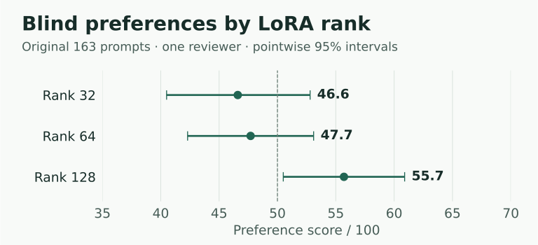
Research noteI had a slight preference for rank 128, though it wasn’t statistically significant. In hindsight, this wasn’t the most useful experiment, but the SFT runs were cheap enough that I ran it anyway.
Experiment 5. Persistent workspace
I switched to mini-SWE-agent so the model could edit files in a persistent workspace. I also removed the refusal tool and asked Luna to leave out text unless the prompt called for it.
Direct Pycairo API access
I wanted to see how Luna would draw with the full Pycairo API. I took out my ArtCanvas wrapper and had Luna write Python that used import cairo, set up its own drawing surface and context, and saved output.png itself.
I reused the same prompt, “an owl with its wings spread out swooping over a tree.” Luna finished in four turns with ArtCanvas and five in the first Pycairo run. In that first Pycairo run it had to fix API and output-path errors before it could submit. I gave Luna a searchable reference from the installed package. It finished the next run in 11 turns without opening the reference. When I explicitly asked it to look up the API before coding, it did so and finished in six turns. I then clarified where to save the image. On that seven-turn run, the path error went away and Luna fixed a gradient argument before submitting. See the owl runs in the experiment log.
I used 2,276 trajectories from the revised setup to train a new rank-128 adapter.
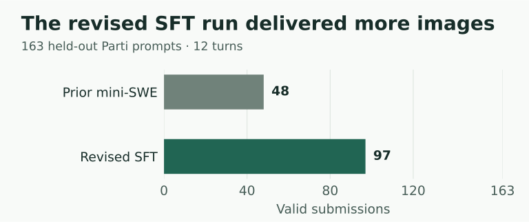
Research noteThe revised checkpoint delivered 97 of 163 images in 12 turns, up from 48 for the prior mini-SWE checkpoint. Average inference tokens per prompt fell from about 118,000 to 75,000. Those figures reflect the combined changes to the drawing API, prompts, tools, and training data. On the 32 prompts both checkpoints finished, HPSv3 leaned 17–15 toward the prior one.
Experiment 6. Loss masking for failed edits
I kept failed edits and repairs in the demonstrations, then trained a version that masked a Python write if its shell command failed. When a preview failed and I could identify the source by its hash, I also masked the writes since the last successful preview with a recorded source hash. The model could still see those writes, learn from the diagnostics, and train on the repair. I trained both adapters from scratch on the same 2,269 trajectories for 71 updates. Both versions delivered 56 of 163 images at the 12-turn cap.
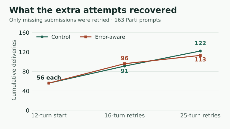
Research noteI kept the simpler loss setup. Both checkpoints delivered 56 images at 12 turns, and HPSv3 favored the control 14–8 on the 22 prompts both finished. After the failure-only retries, HPSv3 favored the control 52–37 on 89 shared deliveries.
Reinforcement learning with verifiable rewards (RLVR)
Experiment 7. Prompt revision and rollout batch sizes
Of 107 failures in the Experiment 6 control, 62 never attempted a preview and 45 had already rendered one before running out of turns. I revised the instructions to describe the drawing workflow more explicitly, including when to preview and when to submit. The planned comparison of the old and new prompts never ran.
For the RL runs, I went back to ArtCanvas. I started from a separate rank-128 SFT checkpoint trained on 2,282 Luna trajectories, with supervision on executed editing actions. The 2,282 traces included PNG observations and had not been human-reviewed. The run took 72 updates and recorded 8,273 supervised actions.
For reinforcement learning with verifiable rewards, I saved the submitted Python and reran it in a clean environment. Missing or invalid images incurred a large penalty. Tool errors incurred a smaller one. A clean submission scored zero. I subtracted 1 for a missing or invalid final image and 0.025 per malformed tool call or failed execution, up to four penalties of each kind. An episode with no tool calls incurred one tool penalty. I used group relative policy optimization (GRPO) with four rollouts per prompt, so each drawing attempt could be compared with the others for the same request. The two batch sizes, 32 and 128 rollouts per update, each used the same 227 Parti prompts and 908 total rollouts. At eight prompts per update the small batch took 29 updates. At 32 prompts per update the large batch took eight.
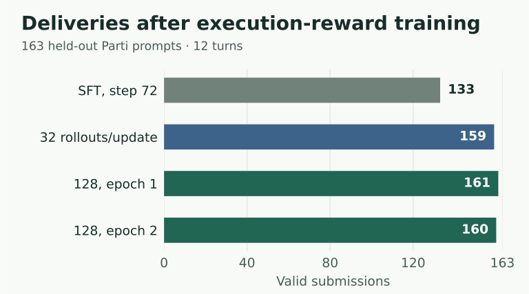
Research noteAfter one epoch, the larger batch delivered two more images, and HPSv3 favored the smaller batch 82–75 on the 157 prompts both finished. A second epoch with the larger batch delivered 160 images, down from 161.
Experiment 8. Expanded RLVR and hard GenAI-Bench evaluation
I started again from the same SFT checkpoint and added 454 GenAI-Bench prompts to the training pool, giving me 2,724 rollouts over 22 updates. I sampled at temperature 1 with a learning rate of 0.00001, PPO clipping at 0.2, and a KL penalty of 0.01 against the frozen SFT model. I tested on 150 screened, held-out prompts covering counting and binding, spatial composition, and comparison and logic. At 25 turns, base, SFT, Parti-only RLVR, and expanded RLVR delivered 108, 109, 141, and 147 images.
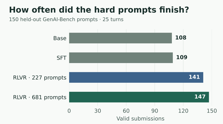

Research noteSFT delivered one more image than the base model, and HPSv3 preferred the SFT drawing on 70 of the 74 prompts both finished. Expanded RLVR delivered six more images than Parti-only RLVR, and HPSv3 favored it 70–68 on shared deliveries. Against SFT, expanded RLVR delivered 38 more images and split the HPSv3 comparisons 53–54. That split gave me a reason to try an image reward next.
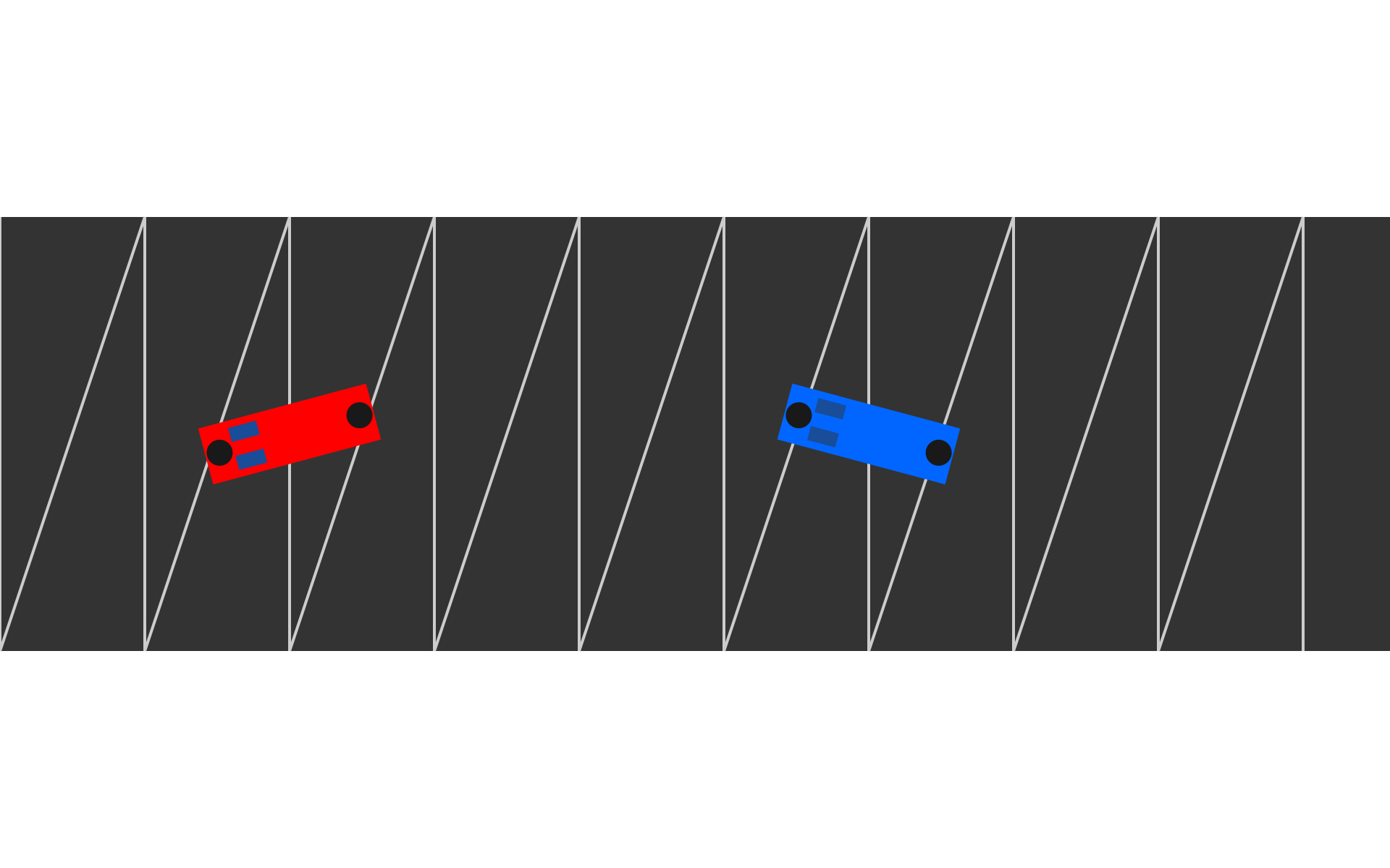
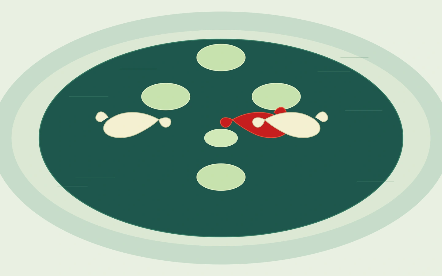
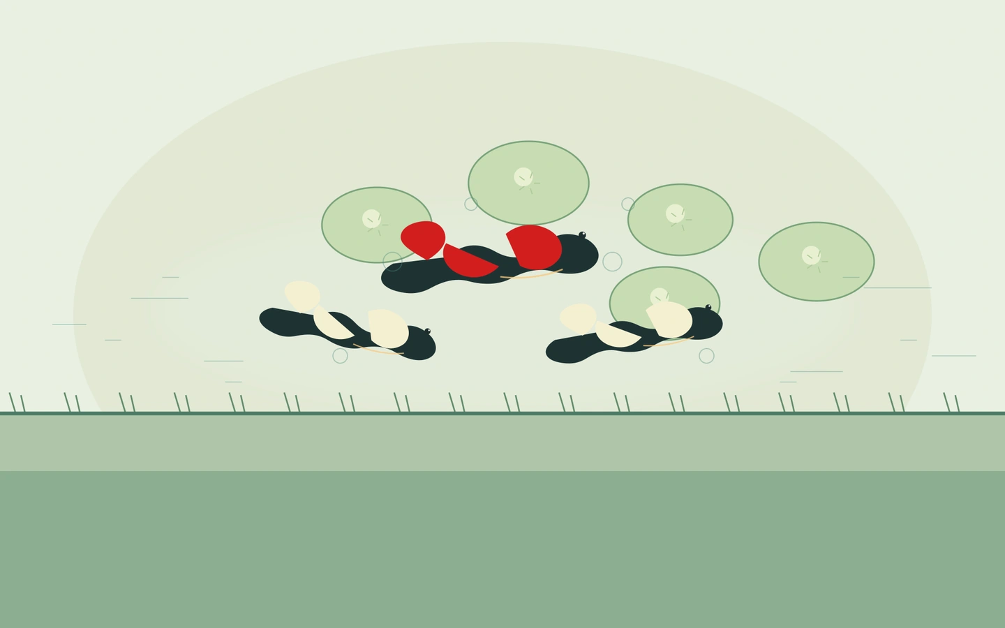
The koi pond lets you inspect what each checkpoint submitted for one prompt. The drawing asks for three fish and specifies their positions relative to the lily pads.

Full prompt
Draw an overhead illustration of a dark teal koi pond. Show exactly three koi: one vermilion fish swimming inside a ring of five pale lily pads, with two ivory fish swimming outside the ring. The fish should have curved bodies and visible fins. Add a few thin ripples and reflections. Use a restrained printmaking style and leave open water around the scene. No text.
Preference-based reinforcement learning
Preference reward pilot on 300 prompts
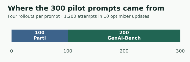
I started from expanded RLVR and changed the reward. A valid image received a normalized HPSv3 score for its prompt. The valid-image reward was 0.02 + 0.98 × clip((raw + 11) / 14, 0, 1), which maps the raw range −11 to 3 onto 0.02 to 1. An invalid or missing submission received zero. HPSv3 supplied the preference signal without new human ratings for each rollout. The first branch used 300 prompts, 1,200 rollouts, and 10 optimizer updates.
Experiment 9. Training on 1,000 prompts and checkpoint recovery
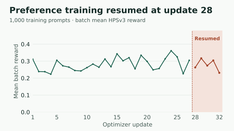
I kept the original 300 prompts, added 700 screened prompts, and started a fresh preference run from the same expanded RLVR checkpoint. The full run used 4,000 rollouts over one epoch, with the same learning rate, group size, clipping, and SFT reference as expanded RLVR. I ran up to 32 Docker episodes at a time. After 27 of 32 updates, KL-reference scoring hit the 262,144-token context limit because the SDK needed one token for output. I lowered the prompt budget to 262,143 and restored the optimizer and data position from update 27. The recovery run covered 544 rollouts across the five remaining updates, completing update 32.
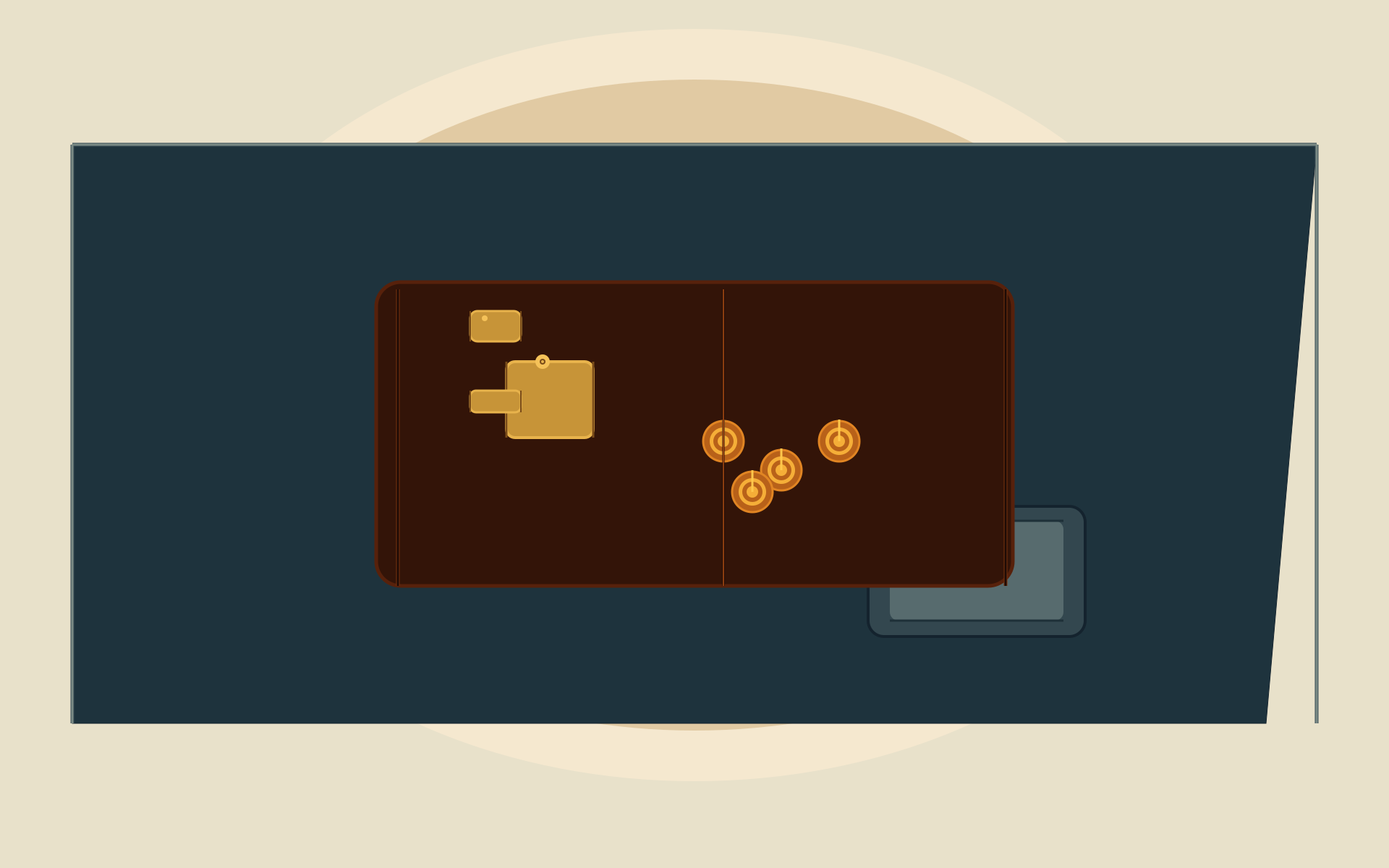


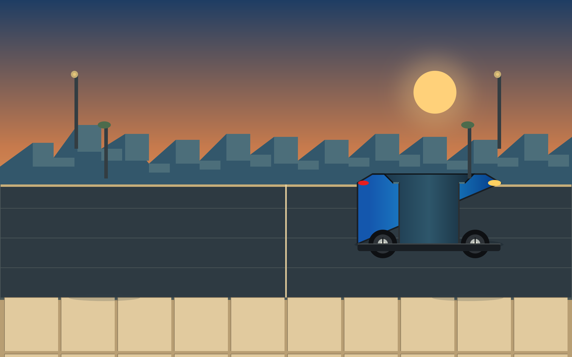
The blood orange and matchbox pairs each use the same prompt, seed, and turn limit. Pick the drawing you prefer before revealing which checkpoint made it.
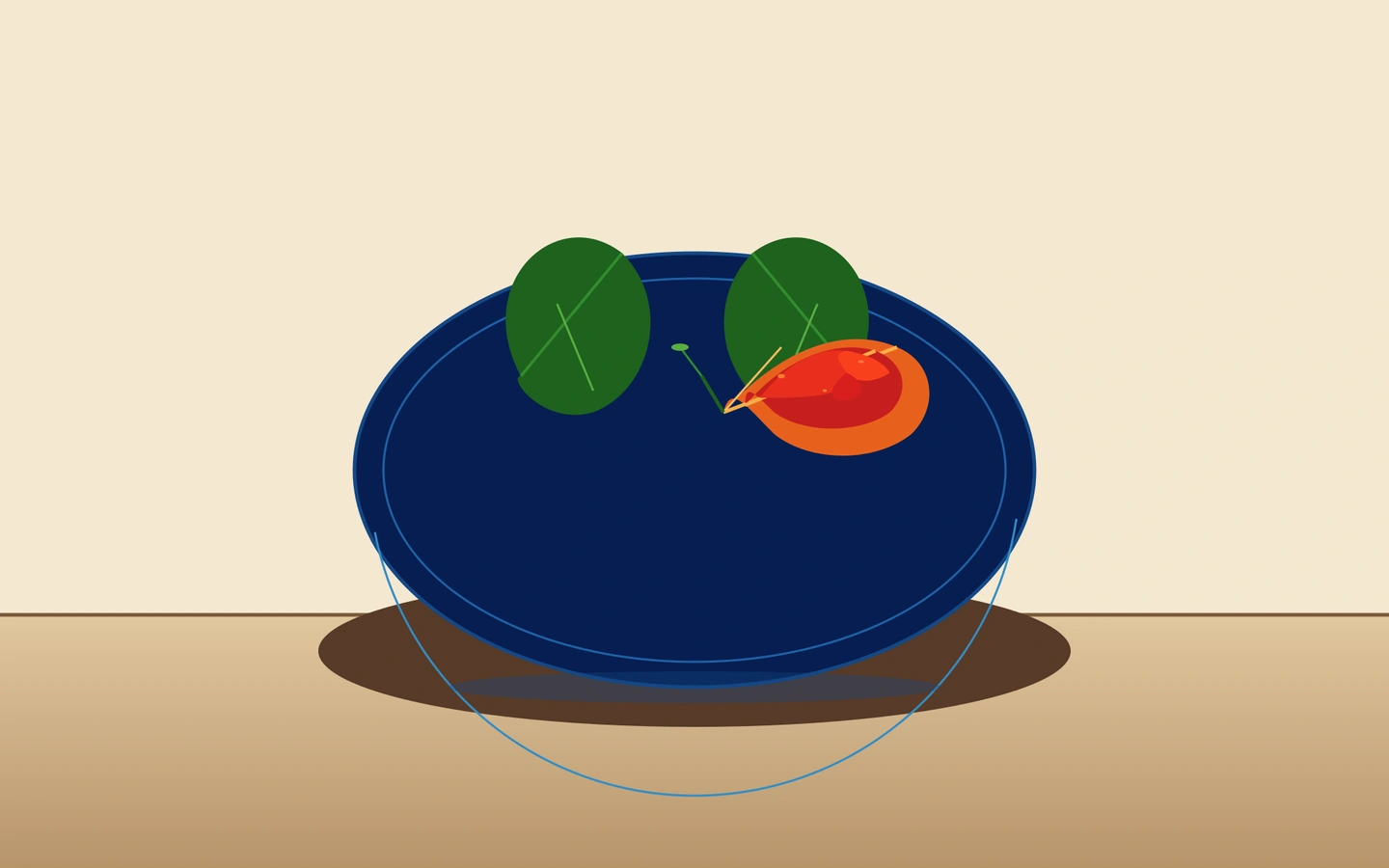
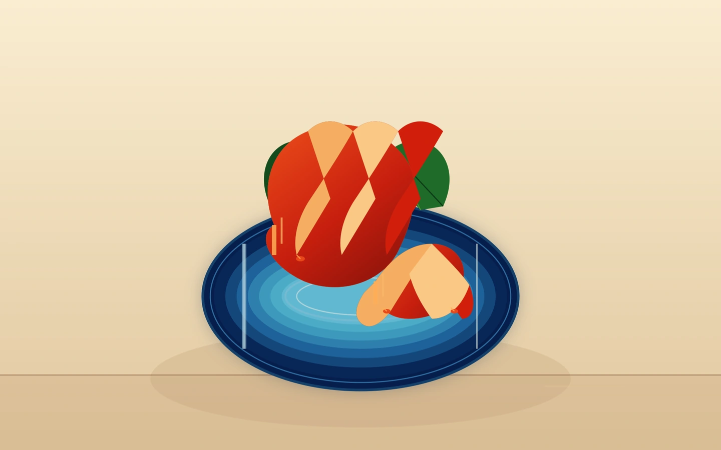
Full prompt
Draw a still life of a blood orange cut in half on a cobalt blue plate, with one wedge in front and two green leaves behind it. Show the cross-section facing the viewer, with visible deep-red segments and a pale rind. Use an angled tabletop with soft shadow, warm cream background, and a bold limited palette in the style of a screenprinted food illustration. No text.
Final checkpoint comparison
I evaluated all five checkpoints with the same 150 hard GenAI-Bench prompts, the same mini-SWE harness in Inspect, and 12 turns each. Each model got one attempt per prompt at temperature 0 with matched prompt seeds, up to 32,768 generated tokens per response, and no combined token or wall-clock limit for the episode. The chart tracks valid submissions and mean normalized HPSv3, with a zero for every failure. Pairwise comparisons use raw scores on prompts where both checkpoints delivered.
Research noteExpanded RLVR and the 1,000-prompt preference run both delivered 149 of 150 images. Mean HPSv3 rose from 0.440 to 0.539, and HPSv3 preferred the final model 96–52 on shared deliveries. The final model also won 75–43 against SFT and 99–2 against base. The two preference runs were nearly even on shared deliveries (72–71). I used the same quantized HPSv3 scorer (mlx-4bit-g64-v1) for training and evaluation.
The biggest gain in valid submissions was on spatial prompts. The base model finished 30 of 50, SFT finished 42, and expanded RLVR and both preference runs finished all 50. This counts whether the drawing rendered. Checking whether it got the requested positions right takes a separate look at the image.
The larger preference run’s higher average came with six more valid submissions than the 300-prompt run. Even on the 143 prompts both finished, the larger run had a higher mean raw score alongside the nearly even win count. My blind review covered the early LoRA checkpoints, so the preference comparison still leaves open which branch people would pick. Each training setting used one seed, so these comparisons describe the checkpoints I evaluated.
The experiment log records the individual runs. The evaluation snapshot includes the chart inputs, source hashes, and instructions for regenerating the figures.